

How replaceable are the top candidates in large hiring rounds? Why the answer flips depending on the distribution of applicant ability
As more and more people apply for a job, the value of each extra application goes down. But does it go down quickly, or only very gradually?
This question matters, because for many of the jobs we discuss, lots of people apply and the application process is highly competitive. When this happens, some of our readers have the sense that, if a lot of people are already applying for a job, there’s no point in them applying as well. After all, there must be someone else suitable in the applicant pool already — someone who would do a similarly good job, even if you were to turn down an offer. So, the logic goes, if you take the job, you’re fully ‘replaceable’, and therefore not having much social impact.
By contrast, 80,000 Hours and many of the organisations we help with hiring often feel differently, saying:
- Even when many people would be interested in taking a job, the difference between the best and the second best applicant is often large. So losing your best option would still be really costly.
- Even when you have a large applicant pool, it’s useful to keep hearing about more potential hires, in the hope of finding someone who’ll be significantly more productive than everyone you’re currently aware of.
Which of these positions is correct? I threw together some simple models in an Excel spreadsheet to explore this disagreement.
In short, which picture is correct depends on the distribution of job applicant productivity, in particular, how large the variance in productivity is among the top tail of performers.
If most people are pretty good at the job, and there’s not much difference in ability between them, then assessing more people quickly loses value. But if most people aren’t good at the job, while a minority of people are much better (i.e. variance in output is high), then getting the 1000th job applicant could be almost as useful as getting the 100th, if both are being drawn from the same distribution.
The most surprising thing that jumps out of the spreadsheet model is that when variance in performance among top candidates is high, the more people apply for a position the less ‘replaceable’ the top candidate is. So, rather than a highly competitive application leading to lots of replaceability, as you might expect, it reduces it.
We’re not sure about how productivity is distributed between workers in jobs, however, it seems likely that many of the jobs we discuss have a high degree of variance in output in the tails, because they’re complex, require unusual skill-sets and are easy to mess up. If this is correct, and the model is appropriate, we’d in a regime where additional applications are valuable and losing the top candidate can be a significant problem.
We’re highly unsure about whether this analysis holds, but it at least shows how it could be possible for an application process both to be highly competitive, and for top candidates to not be replaceable.
(Also note that even if someone is fully replaceable in a job, it can still be worth taking it, because doing so frees up the person who would otherwise take that role to do something else high-impact. We don’t discuss this point further in this article, though it’s another reason that the value of taking a competitive job can be higher than it first seems. See our article on comparative advantage for further discussion of this issue.)
Unfortunately I don’t have more time to spend on this project, so this is a brief blog post to report what I observed, and an invitation to readers to play around with the model themselves, and perhaps find empirical data on job performance that might help inform which figures to use.
I’ll start by briefly discussing different possible distributions of productivity, and then introduce the model.
Table of Contents
Some possible distributions of job performance
People vary in how productive they are in a given job. But how, and how much?
For the purpose of introducing our model, we’ll consider two possibilities:
- If job performance is like height, it will fall in a normal distribution. Some people are taller than others, but nobody is ten times taller than anyone else.
- If job performance is like income, or the number of citations people have on academic papers, it is more like a log normal distribution (or a power law, a related and similar distribution which we’ll ignore here for simplicity). That is, most aspiring academics have few citations, while some have thousands, tens of thousands, or even hundreds of thousands.
Here you can see their different shapes. The important point is the log normal has this big or ‘fat’ tail out to the right that the normal curve does not.
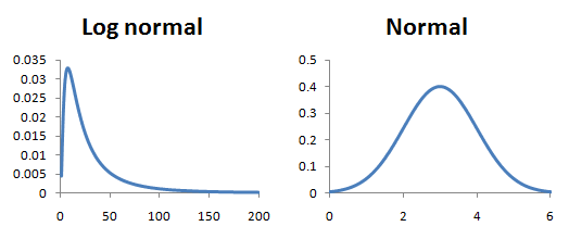
(In reality human height has a right skew and so isn’t quite normally distributed, but it’s close enough to serve as an example.)
How much better does the best applicant get as you review more people? Normal vs log normal
The more people you consider for a role, the better your best option will become. But as you interview more people, you hit declining returns — the odds of finding someone better than the one you already have gets smaller and smaller.
Life is short and nobody wants to interview a million people to find the world’s best employee. At what point does the return to further searching exceed the benefit?
I sampled hypothetical job applicant pools of different sizes at random, to see how the quality of the top candidate would increase as more applications came in.
With a normal distribution the returns to further applicants declines very steeply:
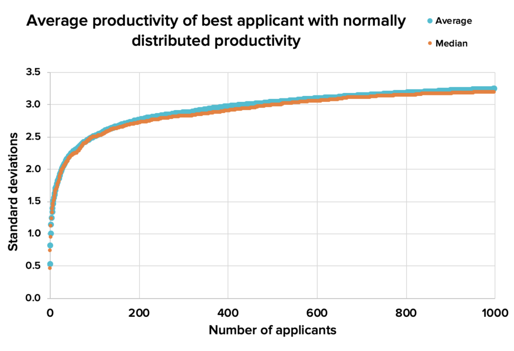
Figure 1. Using a normal distribution of productivity, the best applicant keeps getting better, but at a sharply declining rate. By the time you have 100 applicants, each extra one is increasing the average and median quality of the best applicant only slightly. Download source spreadsheet.
But what if we’re talking about the kind of job where some people are just way better than others?
Taking that same normal distribution, and transforming it into a log normal distribution (e^Normal), makes a significant change to that result. Additional applicants continue to add quite a bit of value, even when you already have a lot of them:
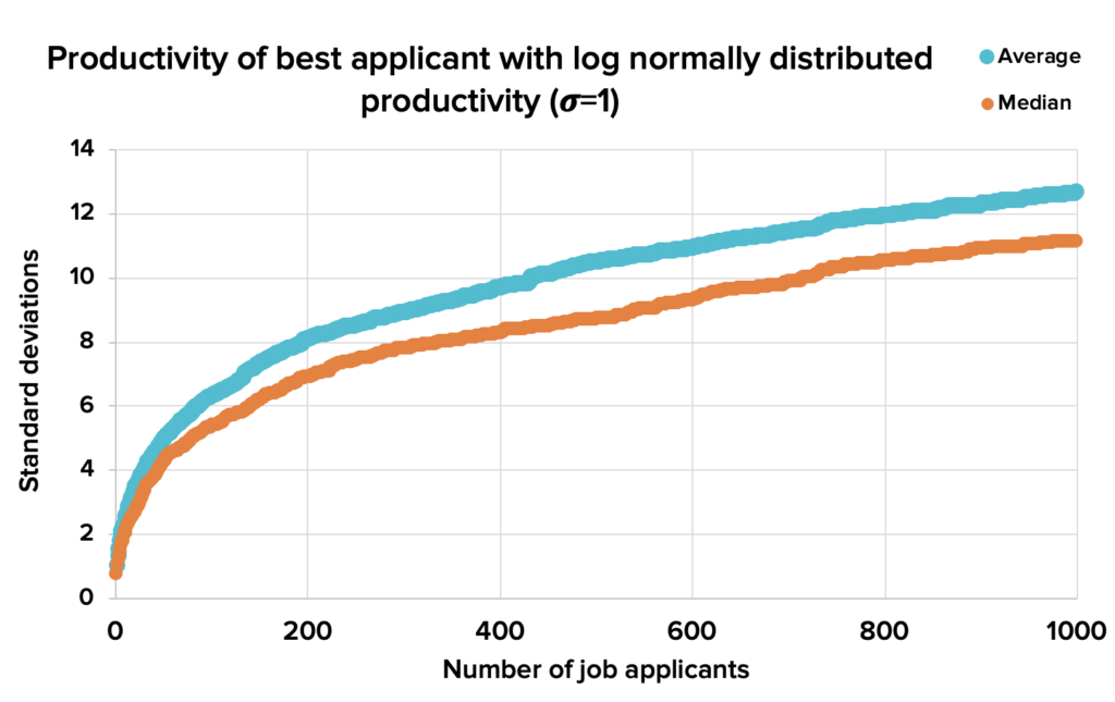
Figure 2. Using a log normal distribution, the quality of the best applicant continues rising even as the applicant pool grows large. Download source spreadsheet.
You’d be forgiven for finding it tricky to tell the difference in shape between those two curves, but here they are lined up against one another:
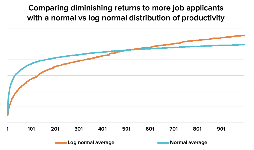
Figure 3. Now we can see that there are much more quickly declining returns to a hiring search with a normal distribution of candidate ability. Download source spreadsheet.
So, the bigger the right tail of exceptional performance, the more valuable it is to keep looking for that perfect hire. So far, so sensible!1
How bad is it to lose your best job applicant?
Alright, so that’s how much an organisation might expect to gain from getting more people to enter their hiring process, if they’re continuously drawing at random from a broad pool.
What about how precious their top applicant in the pool is?
Some people feel that if you have a lot of folks interested in a role, it shouldn’t be a big deal if the best applicant decides not to work there. The next best candidate should be almost as good. And if you’re drawing from a normal distribution they’d be exactly right:
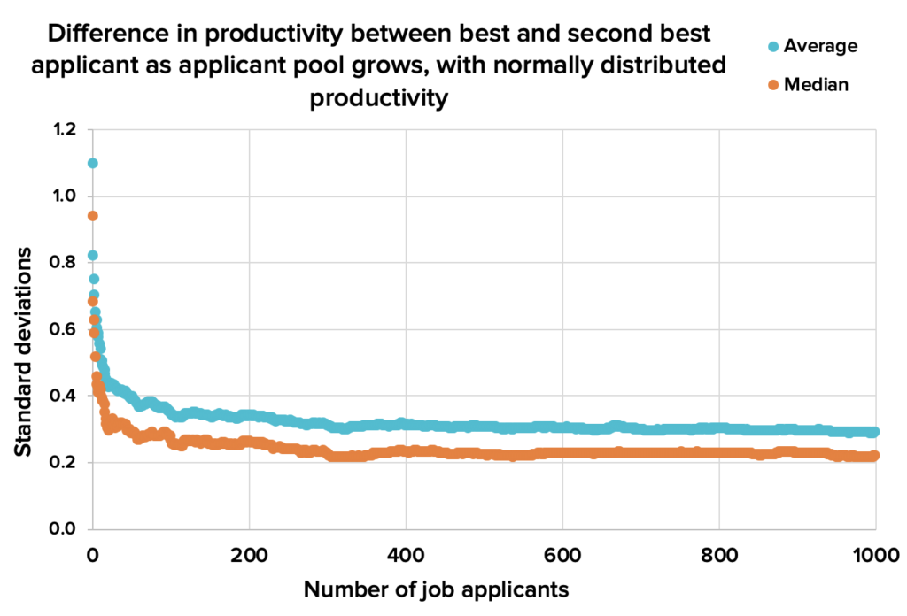
Figure 4. With a normal distribution, the difference in how good the top two job applicants are declines quickly, levelling out at around 0.3 standard deviations. So the loss of the best applicant is typically only a modest setback. Download source spreadsheet.
But organisations we’ve spoken to sometimes feel differently. If their top candidate turns them down, they often feel it’s a significant set-back, and it can sometimes cause them to decide to simply not fill the position at all.
And if applicant productivity is distributed using the same log normal distribution as before, this is just what you should expect them to say. It’s peculiar, but with our log normal distribution of job applicants, the top applicant becomes less and less ‘replaceable’ — they stand out ever more from the rest of the candidate pool.
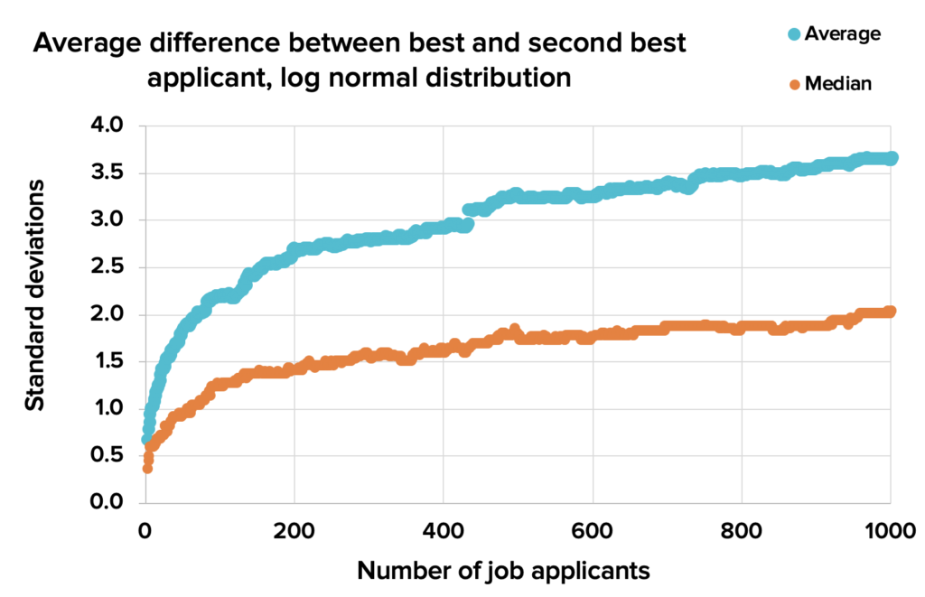
Figure 5. With a log normal distribution, the difference between the top two candidates increases rather than decreases, as more people apply. Download source spreadsheet.
There are two competing effects here. On the one hand, as we add more applicants to the pool, there are more candidates who might be nearly as good as the top one. But as we add more applicants, we also increase the likelihood that the top candidate is a superstar drawn from the long right tail who’s much better than everyone else in the pool. With the parameters we’ve used to generate this distribution, the second effect dominates.2
We spoke to one organisation which said they had a different impression. They said that they thought they had lots of similarly good candidates, and on the margin it was hard to choose between them.
But in that case, rather than hire one person, they were trying to hire ten people from a large applicant pool all at once. With a log normal distribution the difference between the tenth and eleventh best applicants is only a 20th as large as the difference between the best two people in the pool. With smaller differences like this, it becomes much harder to decide who should narrowly be accepted, and who should narrowly be rejected.
So in fact, they were observing what both a normal and log normal distribution of applicant ability would have predicted.
(What if we play with the underlying normal curve we’re using as an exponent to generate our log normal distribution? Increasing the mean just shifts everything up proportionally, and so doesn’t change the differences. Lowering the variance gradually makes the log normal curve converge back to a standard normal curve. Raising the variance makes the top tail longer, and eventually makes the difference between the top two candidates increase nearly linearly.)
Does this imply anything in real life?
It seems like this provides potential support for organisations doing pretty extensive searches to fill roles, and for readers to apply for jobs, even if they’re very competitive. But before we go there, we should list some qualifications:
- Are the tails of performance closer to a normal distribution or log normal distribution? We’re very unsure about this question, and would like to see more research into it. Some evidence we’ve seen suggests that output is normally distributed even in ‘complex’ jobs, like being a doctor. However, for the most difficult and creative work, like academic research, we suspect that the variance is high in the tails. Even there, it’s hard to be confident since many measures of output (such as citation count) are likely to overstate differences in productivity.
As more people apply for a role, the bar for being the best candidate goes up. Assuming a normal distribution, if only ten people have applied for a job, you have a 10% chance of being the best option by being just 1 standard deviations above the average. But if 100 people apply for the same position, you’d have to be 2 standard deviations above average to have that same 10% chance of being the top candidate.
We generally encourage people to take an optimistic attitude to their job search and apply for roles they don’t expect to get. Four reasons for this are that, i) the upside of getting hired is typically many times larger than the cost of a job application process itself, ii) many people systematically underestimate themselves, iii) there’s a lot of randomness in these processes, which gives you a chance, even if you’re not truly the top candidate, and iv) the best way to get good at job applications is to go through a lot of them.
But despite all that, it’s worth keeping in mind that as more people take an interest in a position, the minimum bar for having a realistic shot at getting hired rises pretty quickly, while the costs to you stay the same.
The model assumed that as an organisation worked to increase the number of applicants it received, the new ones were being drawn from the same pool as the old ones. This is obviously questionable, though I’m not sure in which direction.
If the best applicants are already busy in high-powered roles and need to be cajoled into applying for anything else, then this counts in favour of a more aggressive hiring process that involves specific headhunting.
On the other hand, if the applicants with the best personal fit apply early, and the people who have to be pushed to apply are sensibly self-selecting out of the process, then this counts in favour of a shorter process.
Even if productivity in a given role across the whole population is very variable, or log normally distributed, this doesn’t mean that will be true among people who actually apply. People who would be especially bad in a role likely won’t even consider it. And people who are so talented as to be overqualified probably won’t apply either, as they’ll be looking for a more senior position. If these effects are large, the differences between applicants at the top might be much smaller than we would naïvely expect.
If you’re an organisation scaling up, you may be hiring quite a lot of people. If you’re hiring people faster than your plausible applicant pool is growing, then the differences between top applicants will shrink over time, as you pick off the best ones first. This is just the same situation as the organisation which was trying to hire ten people all at once, but spread out over time.
Finally, we haven’t considered the costs of applications to the applicant or the organisation they’re considering working at. If applying for a role absorbs a material fraction of the time you’d expect to spend in the job before moving on, then you should consider far fewer positions.
At 80,000 Hours we always trial people before hiring them, which absorbs days of their time and our time. There are benefits to both sides of gathering so much information about one another, but with such an involved application process, you only get to consider a smaller number of roles and people respectively.
The model doesn’t consider measurement error on the part of people assessing applicants. I suspect that will push all values in the graphs above closer to zero, probably multiplying them by some fixed factor that’s less than 1. This would be a good thing for someone to test if they wanted to explore further. (Update: I made a spreadsheet to test this intuition, introducing a measurement error where an organisation’s assessment of someone productivity is their true productivity multiplied by a random log normal that typically ranges from 0.4 to 2.2, and indeed it seems to be right.)
Summing up
I started playing with these figures to answer two questions in my mind:
- How quickly does it stop being worth searching for better potential hires?
- Why do organisations who could hire from a large pool of interested candidates nonetheless feel that losing their top candidate would be very bad?
The answer to the first question depends on how widely distributed ability is. If it’s distributed normally, a small search is likely sufficient. If it’s very unequally distributed, a more comprehensive hiring process can be justified, and candidates who think they might be excellent in the role should apply even if hundreds of others already have.
I also identified a potential answer to the second question. If ability is distributed log normally — which it may well be for some kinds of positions — then it should be common for organisations with many potential hires to vastly prefer one of them. But it’s also possible folks are simply mistaken and the second-best candidate is better than they think.
As always, there are ways this model could fail to match reality, some of which I’ve described above.
The arguments about whether job productivity is normally or log normally distributed, and how that differs across role type, are complicated enough that we decided not to include them in this post. However, we hope to write more about them at some point in the future.
Appendix – Some final thoughts for researchers
I’ve made all the spreadsheets I used for this analysis public and fairly easy for other people to use, as I expect someone could turn up some interesting findings by playing around with them. (1, 2, 3, 4)
I have some statistical training, but not enough to prove anything interesting about the properties of log normal distributions, let alone something more complicated. Fortunately, I can go a long way without anything like that. With a mere spreadsheet, or some simple programming in R, anyone can randomly draw points from a statistical distribution, perform a series of calculations on them, and inspect the shape of the results.
This seems like an underutilised method of building rough models of the world. In fact, it can allow you to build more realistic and messy models than more formal methods. Let’s say that I wanted to see how the picture changes if the distribution of ability is a mixture of a normal and a log normal distribution. Someone trying to develop mathematical proofs will find this fairly tricky. But in Excel it’s trivial — I just draw a random normal, a random log normal, add them together, and carry on with the rest of my calculations. So if you feel so inclined, experiment with building out the sheets I put together and let me know what you find.
Notes: Thanks to Howie Lempel, Ben Todd, Roman Duda and Denise Melchin for feedback on drafts of this piece.
Notes and references
- This model assumes that applicants are equally good whether they apply early or later on. It might be natural to expect that the most suitable candidates are likely to apply first, with later applicants who have to be cajoled into participating having worse fit for the role. However, we’ve often found that the best candidates have to be strongly encouraged to apply, either because they’re busy with other projects, or because they don’t fully appreciate their own abilities.↩
- Experimenting with the ‘fatness’ of the log normal distribution we find that by setting the parameter sigma to 0.4, the difference between the best and second best applicant remains constant as the applicant pool grows.↩