

Estimation – Part II: How much will you earn?
What can we use estimates for?
How much could I earn during my life as a lawyer? How many people could this campaign reach? How long will it take to complete this research? There are lots of figures that would be extremely useful to planning your career, but that are highly uncertain. Rather than making a direct estimate, it’s better to break these questions down into a number of sub-questions.
For these sub-questions we can use the four techniques (the equivalent bet, the absurdity test, avoiding anchoring and listing pros and cons) learnt in Part 1 of this post to make calibrated Confidence Intervals (CIs).
We can then combine these individual estimates to answer our original question, and once we have done this for a number of different options we can compare them to make decisions about our future career.
In the following post we will therefore be looking at:
* How we can combine individual estimates to answer complex career questions
* How to compare different career options.
* How we can improve our estimates
Combining estimates
In order to look at how to combine estimates we will consider the question posed above; ‘What are my expected lifetime earnings if I choose a legal career?’
After a bit of thought we decide that in order to create a simple linear model for this calculation we need to know how much is the initial salary at the graduate level, final salary at the executive level and how long it will take for us to progress from the graduate level to the executive level. For now we are going to ignore other factors such as how likely I am to get to the top of my firm and historic trends in pay levels.
We have already looked at ways to find out salary information in another blog post and following from this we used information from Salary.com to make a number of 80% CI’s for the numbers we are interested in:
* Graduate Lawyer: $66,024 – $129,064
* Top Legal Executive: $195,145 – $728,587
* Time to reach top salary: 5 – 30 years
A model1 for calculating Lifetime Earnings might split our career into two phases, one where our salary is increasing as we progress towards the executive level, and a second phase where our salary stays at executive level.
How do we combine these figures when each variable is a range, as is the case with our 80% CIs, instead of a single value.
First we might think of just picking the median value of each CI. In this case our lifetime earnings would be $15,000,000. But as we mentioned in Part 1 a single value isn’t of much use as it doesn’t give us any information about our level of uncertainty and is very unlikely to be correct.
We could put the best and worst values for each sub-estimate into two separate calculations and then use the answers to these as the upper and lower bounds for the overall 80% CI of lifetime earnings? This also turns out to be a bad idea as the final range often ends up being too wide, particularly in more complex problems with more variables, due to the fact that most of the time we will get a combination of all the values, some high, some low, rather than expecting to routinely get all values as either high or low2.
In fact the best way to combine estimates is to use the Monte Carlo Method3. This method involves picking a number at random from within each range and performing the calculation. You then pick new numbers and repeat the calculation. By doing this thousands of times you can examine your results to see the final distribution for your original question. More information on this method can be found in the notes1 at the end of this page as well as ‘How to Measure Anything’4.
We have carried out a Monte Carlo Simulation for the expected earnings in a legal career, the results of which can be seen in the graph below.
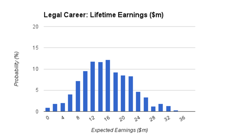
By performing these calculations we provide ourselves with as much information as we can when it comes to analysing our results. From the data we know that the mean lifetime earnings are $15.4m and that our 80% CI is $6.8m to $24.4m. We also have the option of combining this distribution with other estimates we have made if we are trying to answer an even more complex question.
Ways of comparing estimates?
In the case of earning to give we will want to compare the expected lifetime earnings for a legal career to one of our other options, in this case a financial career5.
We could pick out single values, such as the mean or median, and compare these, but this doesn’t take into account the uncertainty in our estimates. One useful figure would be the probability that earnings are greater for a legal career than for a financial career.
In this example the expected earnings for a legal career are $15.4m and for a financial career they are $19.5m, we also know that there is around a 35% chance (according to this model) that we will earn more if we choose a legal career than if we choose a financial career.
With these results we would choose to take up a career in the financial industry and we know that we have a 65% chance that we are making the right decision. We might ask ourselves whether this is an acceptable level of confidence to have for such a big decision?
Can we improve our estimates?
At the moment we have a 65% level of confidence that we will make the right decision if we go into banking. For any model it is possible to improve the accuracy of results by following two courses of action:
* Increase the level of detail of the model.
* Reduce the uncertainty of our individual estimates.
In the case of earning to give we might increase the level of detail by taking into account factors such as historical salary variation or the probability of being promoted at each level based on our ability. In order to reduce our uncertainty we might be able to narrow the range for some of our 80% CIs. This means that when we select values for our Monte Carlo Simulation they more accurately reflect the actual outcome, and this follows through to increase the accuracy of our final estimate.
The problem is that increasing our confidence takes additional time and, possibly, money. The key question is ‘Is it worth spending this extra money in order to increase our chances of making the right choice?’ Working this out properly requires a Value of Information calculation which we will be covering in a future blog post.
30/04/13 UPDATE: Original post was missing the graph of expected earnings, this has now been included.
You may also enjoy
Notes and References
- The mathematical model used to calculate lifetime earnings was: LE = (S1+S2)T1/2+(40-T1)S2 ↩ ↩
- Some other methods may circumvent this problem but they often have problems adding or multiplying ranges which use different distributions. ↩
- The Monte Carlo method
The Monte Carlo method is a ‘brute force’ computing method, where thousands of different calculations are carried out to provide thousands of different answers. By analysing the distribution of these answers we can then work out the probabilities of the different outcomes.
One of the most important things with a Monte Carlo simulation is to ensure that we are selecting the right numbers to plug into our calculations. To do this we treat each variable as a different statistical distribution, and use a spreadsheet to randomly select the numbers within these distributions. As each distribution has different properties we need to choose them carefully to ensure that they suit our different variables. Some commonly used distributions are the Normal, Log-Normal Binary and Uniform Distributions, information on their characteristics as well as their applications can be found in How to Measure Anything (see below). ↩
- Hubbard, D. W. (2010) Calibrated Estimates: How much do you know now? In How to Measure Anything, 2nd Edition, Hoboken: John Wiley & Sons, Inc. ↩
- the monte carlo simulation for lifetime earnings in a financial career can be found at https://docs.google.com/spreadsheet/ccc?key=0aiktarl7q4lcdezazhrkbhfxtm15s1zqeg1hu2dxr0e#gid=2. ↩